Quantization Fundamentals for Multi-Vector Retrieval

Multi-vector search approaches are now critical for coding agents and multi-modal applications. MixedBread, Cursor, Parallel AI, and others have enabled coding agents to use this semantic search because it cuts token usage in half, allows agents to finish tasks in half the time, and yields better-quality outputs. I’ve validated the impact on my own commercial codebases and analysis.

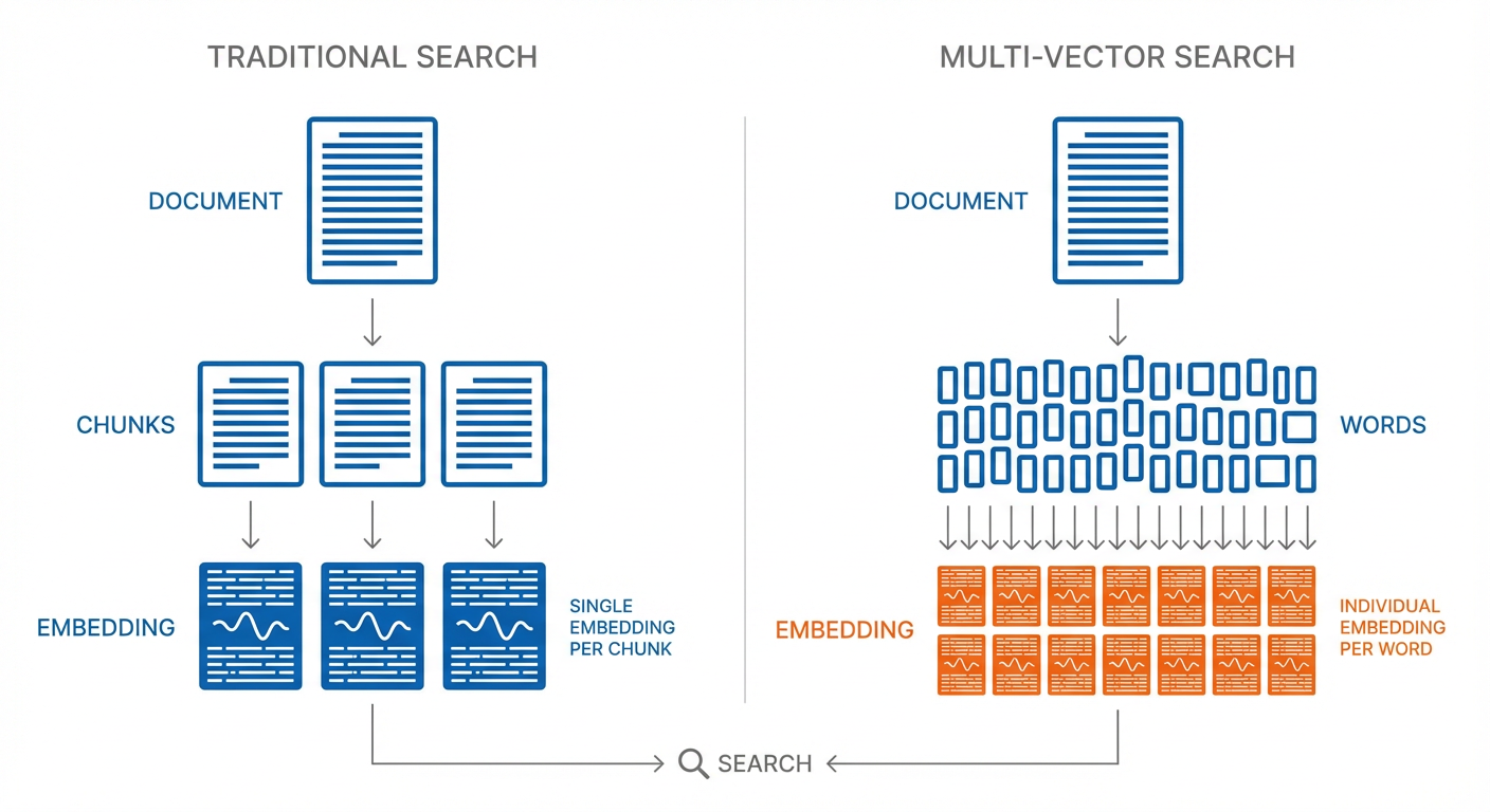
Multi-vector search is more powerful because it uses more contextual data from the inputs. The architecture stores a separate embedding for each word in a document, rather than the traditional approach of storing an entire document (or chunk) in a single embedding. This gives multi-vector approaches a more detailed understanding of the content, but it also means there's a lot more embeddings.

Quantization is what makes handling this extra information practical in many cases. By representing numbers with fewer bits (like rounding to fewer decimal places), quantization trades a small amount of precision for a large reduction in storage.

This post is a guide to understanding how quantization for multi-vector and ColBERT approaches work. Sign up for the talks below to get detailed write ups on other deep dives on usage, architecture, and research about multi-vector approaches beyond just the quantization.

Upcoming Talks on Multi-Vector Search

• Modern Multi-Vector Code Search – Technical deep-dive on the multi-vector approach by mixedbread’s founder
• The 1/2 Token Codebase Search – Benefits and intuition for using multi-vector search with agents to improve speed, quality, and reduce token usage.

Can’t attend live? Sign up for the talks to receive detailed writeups and recordings.

Intro to Quantization

Before diving into the advanced approach ColBERT uses (Product Quantization), let’s understand the basic concept of quantization with a simpler approach.

We’ll start with creating some dummy data to quantize.

# Let's create some example data - a simple sine wave
x = np.linspace(0, 2*np.pi, 100)
original_values = np.sin(x)

We can look at the size of the data we are starting with. Our goal is to reduce the size of original_values without losing too much information. This is called Quantization.

Original values use float64 (64 bits per value)
Total bits: 100 values × 64 bits = 6400

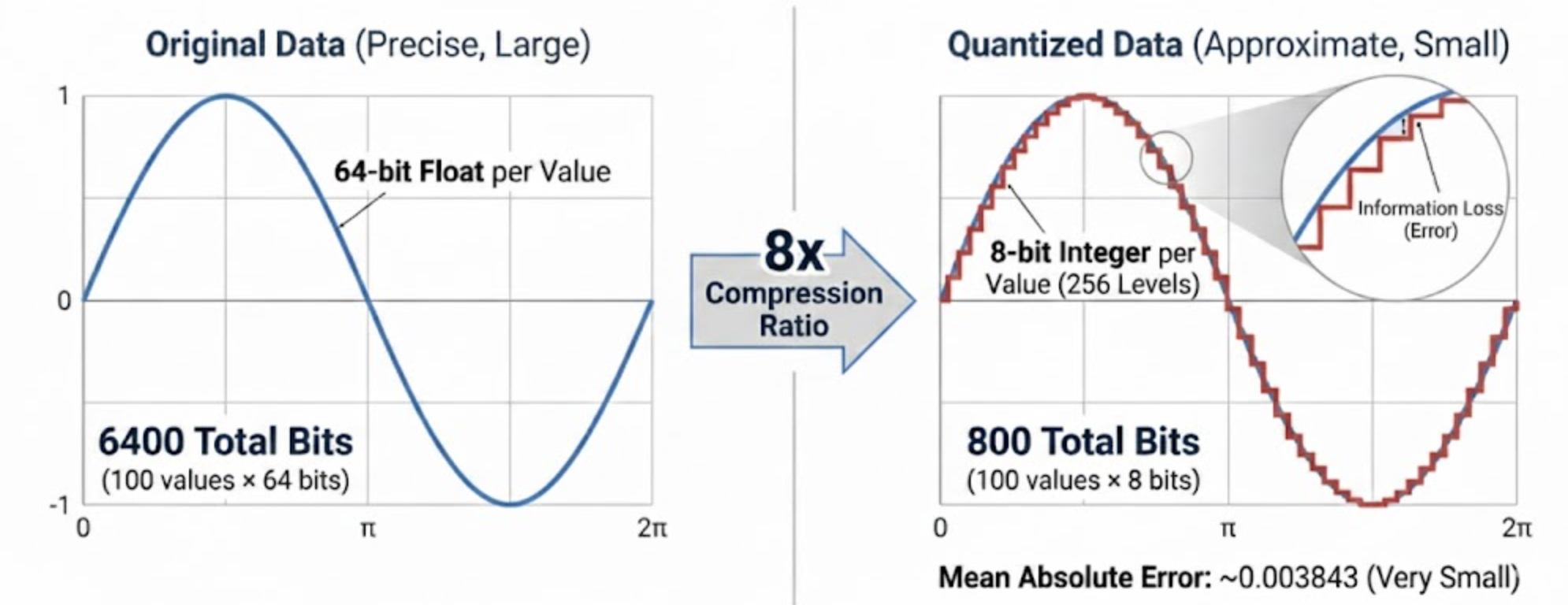
Let’s compress this data so we’re only storing 8 bits per value. All data values are between the minimum and the maximum value. We want to represent each one of them using just 8 bits. We do this by dividing up the range into 2^8 = 256 equal intervals (called levels) and storing which level each value is in.

bits = 8
levels = 2**bits

Let’s save the minimum and maximum values that defines the range we need to divide up.

min_val = np.min(original_values)
max_val = np.max(original_values)

Now we can quantize the data to these levels by replacing the 64 bit data value with the 8 bit level it lies in. We’ll use the astype function to convert the data to the new type. This is a simple form of quantization called uniform scalar quantization.

scaled = ((original_values - min_val) / (max_val - min_val) * (levels - 1)).astype(np.uint8)

This is our quantized representation - just 8 bits per value instead of 64. Much smaller!

print(f"Quantized values use {scaled.dtype} ({scaled.dtype.itemsize * 8} bits per value)")
print(f"Total bits: {scaled.nbytes * 8}")

Quantized values use uint8 (8 bits per value)
Total bits: 800

We can calculate how much space we saved by comparing the original size to the quantized size.

original_values.nbytes / scaled.nbytes

8.0

This is a compression ratio of 8x. We’ve gone from 64 bits per value to 8 bits per value. Not bad!

Great! Now what’s the catch? Well, we’ve lost some information.

We’ve rounded the values to the nearest level. This means that some values are not exactly the same as the original values. Sometimes this is a big deal, but sometimes it’s not.

We can measure how much error we introduced. We’ll use mean absolute error, which is just the average difference between the original and reconstructed values. Quantifying information loss is an important concept to be aware of.

To calculate the error, we’ll need to convert back to the original range. This is the inverse of the scaling we did earlier.

_range = max_val - min_val
reconstructed = (scaled / (levels - 1)) * _range + min_val
mean_absolute_error = np.mean(np.abs(original_values - reconstructed))
print(f"\nMean absolute error: {mean_absolute_error:.6f}")

Mean absolute error: 0.003843

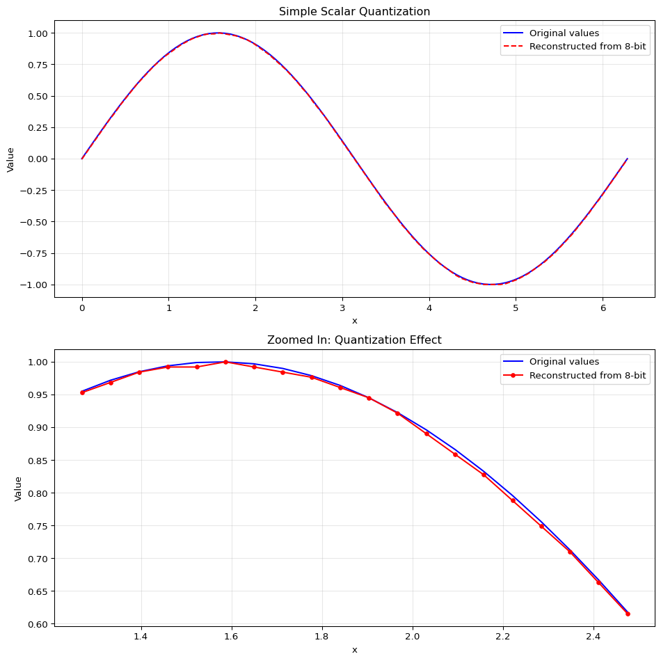
Because our sample data is so simple, we can see the error is very small. We’ll plot the original values and the quantized values. You can see that while it’s almost the same line, our reconstructed values are not exactly the same as the original values. That’s called information loss. We reduced the size of our data from 64 bits per value to 8 bits per value, but we lost some information in the process.

# Visualize the results
fig, ax = plt.subplots(2,1, figsize=(10, 10))
ax[0].plot(x, original_values, 'b-', label='Original values')
ax[0].plot(x, reconstructed, 'r--', label='Reconstructed from 8-bit')
ax[0].set_title('Simple Scalar Quantization')
ax[0].set_xlabel('x')
ax[0].set_ylabel('Value')
ax[0].legend()
ax[0].grid(True, alpha=0.3)
zoom_start, zoom_end = 20, 40
ax[1].plot(x[zoom_start:zoom_end], original_values[zoom_start:zoom_end], 'b-', label='Original values')
ax[1].plot(x[zoom_start:zoom_end], reconstructed[zoom_start:zoom_end], 'ro-', markersize=4, label='Reconstructed from 8-bit')
ax[1].set_title('Zoomed In: Quantization Effect')
ax[1].set_xlabel('x')
ax[1].set_ylabel('Value')
ax[1].legend()
ax[1].grid(True, alpha=0.3)
fig.tight_layout()
plt.show()

This is the most basic form of quantization - uniform scalar quantization. We’re simply:

• Taking continuous values in a range
• Mapping them to a smaller set of discrete levels (like 256 levels for 8-bit quantization)
• Using these discrete levels to reconstruct approximations of the original values

The tradeoff is clear: we reduce storage space at the cost of some precision. With 8 bits, the error is usually very small for many applications.

Quantizing Whole Vectors

We’ve seen how to quantize scalar data, which consists of single numbers. But for ColBERT, we need to quantize embeddings (high-dimensional vectors).

We could still apply scalar quantization to each number independently, but quantization errors add up across all dimensions. Finding quantization parameters that work well across the entire embedding space would be challenging.

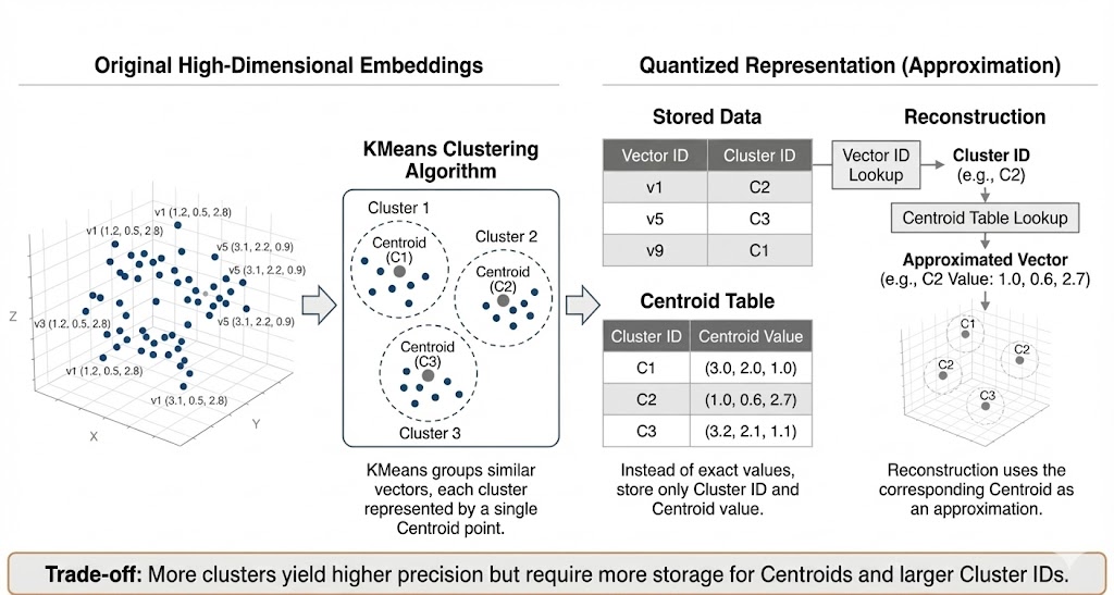
In practice it often works better to quantize vectors as a whole, instead of each number individually. This is done using a clustering algorithm like KMeans to group similar vectors. The algorithm organizes the data so that vectors with high similarity end up in the same cluster. Each cluster is then represented by a single point called a centroid. The key idea is this: instead of storing each vector’s exact values, we store two things:

• The cluster ID that each vector belongs to.

• The centroid value for each cluster.

When we need to reconstruct a vector, we look up its cluster ID and use the corresponding centroid as its approximation. This method provides a good balance, significantly reducing storage space while maintaining a reasonable approximation of the original data. As you might expect, there's a trade-off: using more clusters yields a better approximation but also requires more storage for the centroids and larger cluster IDs.

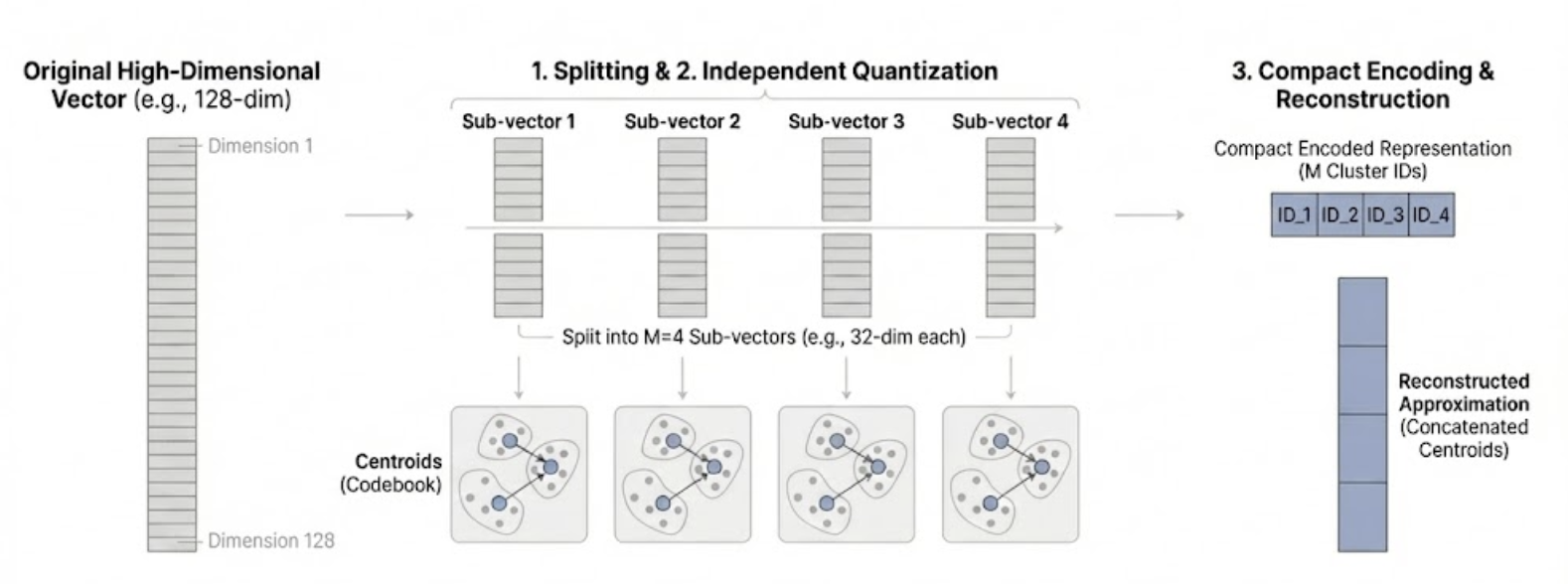
This approach, often called Vector Quantization (VQ), is a solid foundation. However, to achieve high precision, it would require a massive number of centroids, making it impractical for large-scale systems. This is where we employ a more sophisticated method: Product Quantization.

Product Quantization builds on the clustering idea but achieves far better compression by splitting each vector into smaller pieces and clustering those pieces separately.

Simplified Version

Let’s understand product quantization with the simplest possible example. We’ll work with just 5 embeddings, where each embedding is a list of 4 numbers.

# Create tiny dataset: 5 embeddings of dimension 4
embeddings = np.array([
   [5.0, 6.0, 3.0, 4.0],  # Embedding 1
   [1.0, 2.0, 7.0, 8.0],  # Embedding 2
   [4.0, 5.0, 6.0, 7.0],  # Embedding 3
   [2.0, 3.0, 4.0, 5.0],  # Embedding 4
   [3.0, 4.0, 5.0, 6.0],  # Embedding 5
])

Step 1: Split each embedding in half.

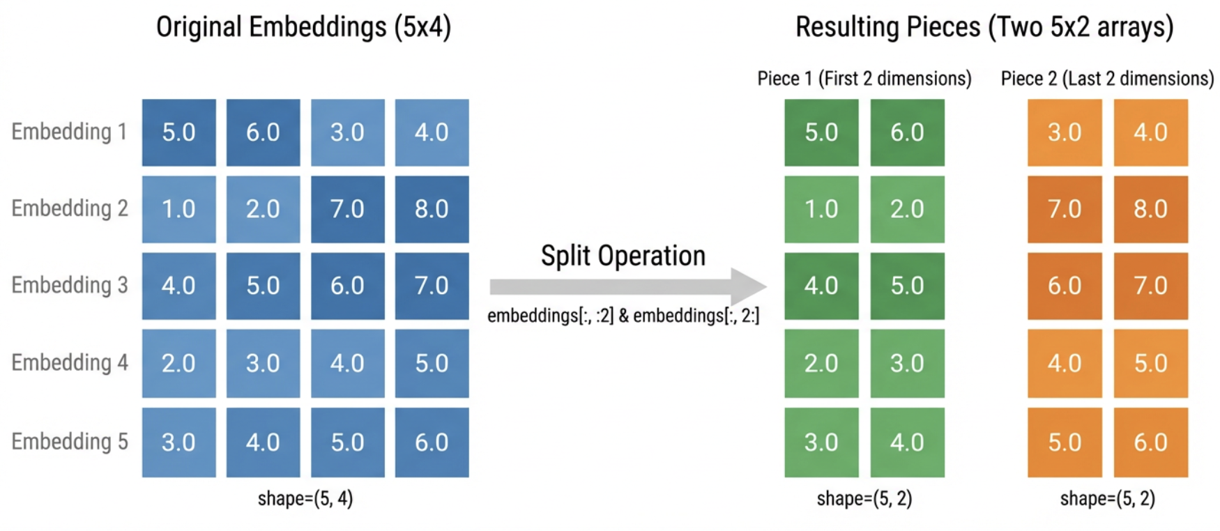
Each embedding has 4 numbers. We split it into two “pieces” of 2 numbers each:

• Piece 1: the first two numbers (positions 0-1)
• Piece 2: the last two numbers (positions 2-3)

For example, embedding [5.0, 6.0, 3.0, 4.0] becomes piece 1 = [5.0, 6.0] and piece 2 = [3.0, 4.0].

piece1 = embeddings[:, :2]  # First 2 dimensions
piece2 = embeddings[:, 2:]  # Last 2 dimensions

We still have all 5 embeddings, but now organized into two separate collections of pieces.

piece1.shape=(5, 2) piece2.shape=(5, 2)

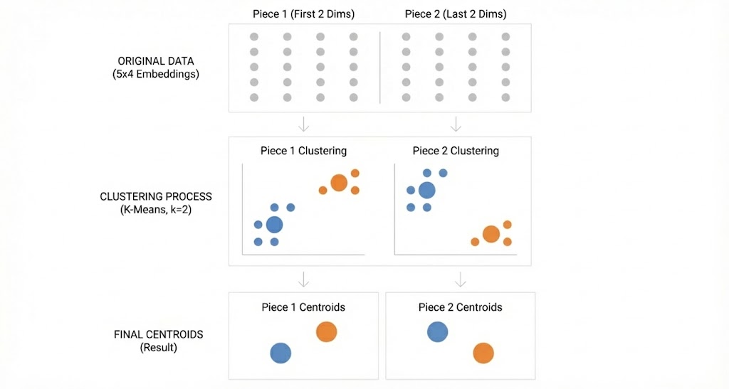
Step 2: Cluster each collection of pieces separately.

Now we cluster each collection. We’ll use 2 clusters per collection. After clustering, each piece gets assigned to a cluster, and we store the cluster’s centroid (the average of all pieces in that cluster).

💡 K Means is a clustering algorithm that is a component of product quantization. If you have no familiarity with clustering and want to understand how it works, check out my previous post for a dive into K Means.

def train_kmeans(piece):
    kmeans = FastKMeans(d=piece.shape[1], 
        k=2, nredo=1, niter=20,
        gpu=False, use_triton=False)
    kmeans.train(piece)
    return kmeans

centroids, indices = [], []
# Use FastKMeans to find centroids for each piece
for piece_index, piece in enumerate([piece1, piece2]):
    kmeans = train_kmeans(piece)
    centroids.append(kmeans.centroids)
    indices.append(kmeans.predict(piece).astype(np.uint8))

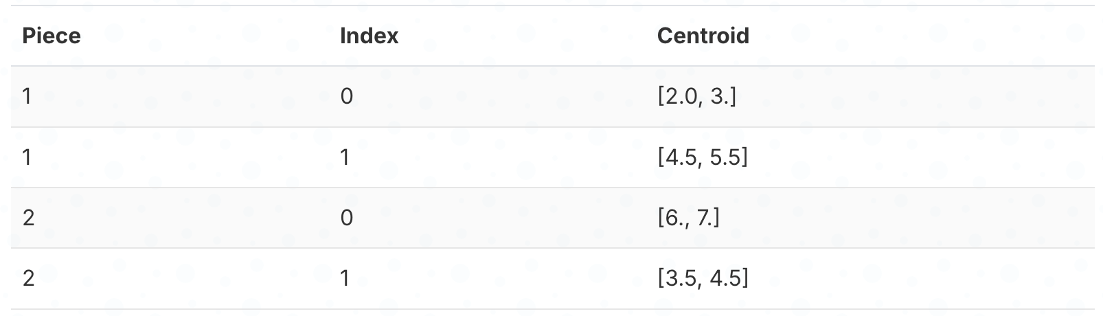
This gives us 2 centroids for piece 1 and 2 centroids for piece 2

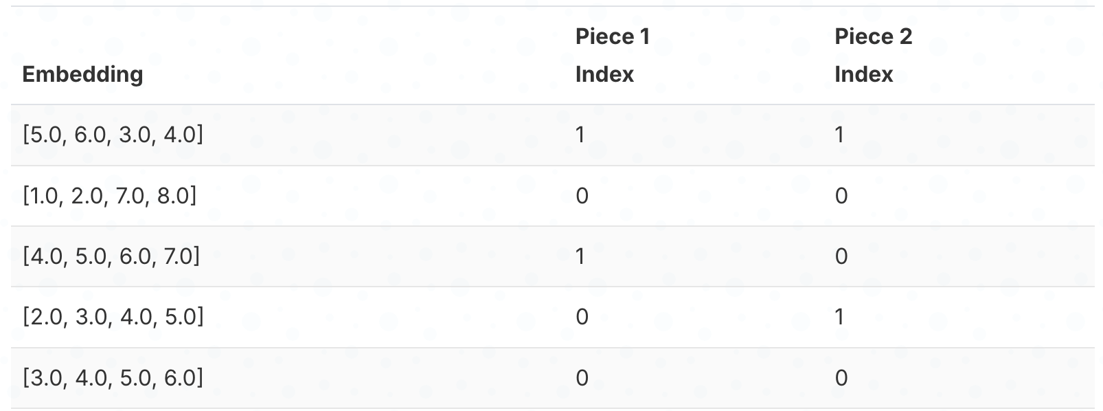
Step 3: Store which cluster each piece belongs to.

Instead of storing the actual numbers, we just store the cluster index (0 or 1) for each piece. We’re replacing 2 floating-point numbers with a single small integer.

💡 You may notice that we are using .astype(np.uint8) like we did in the scalar quantization example for these indices! These indices just tell us which cluster each piece belongs to, and there aren’t very many clusters so 8 bits is plenty.

Here’s which cluster each embedding’s pieces belong to:

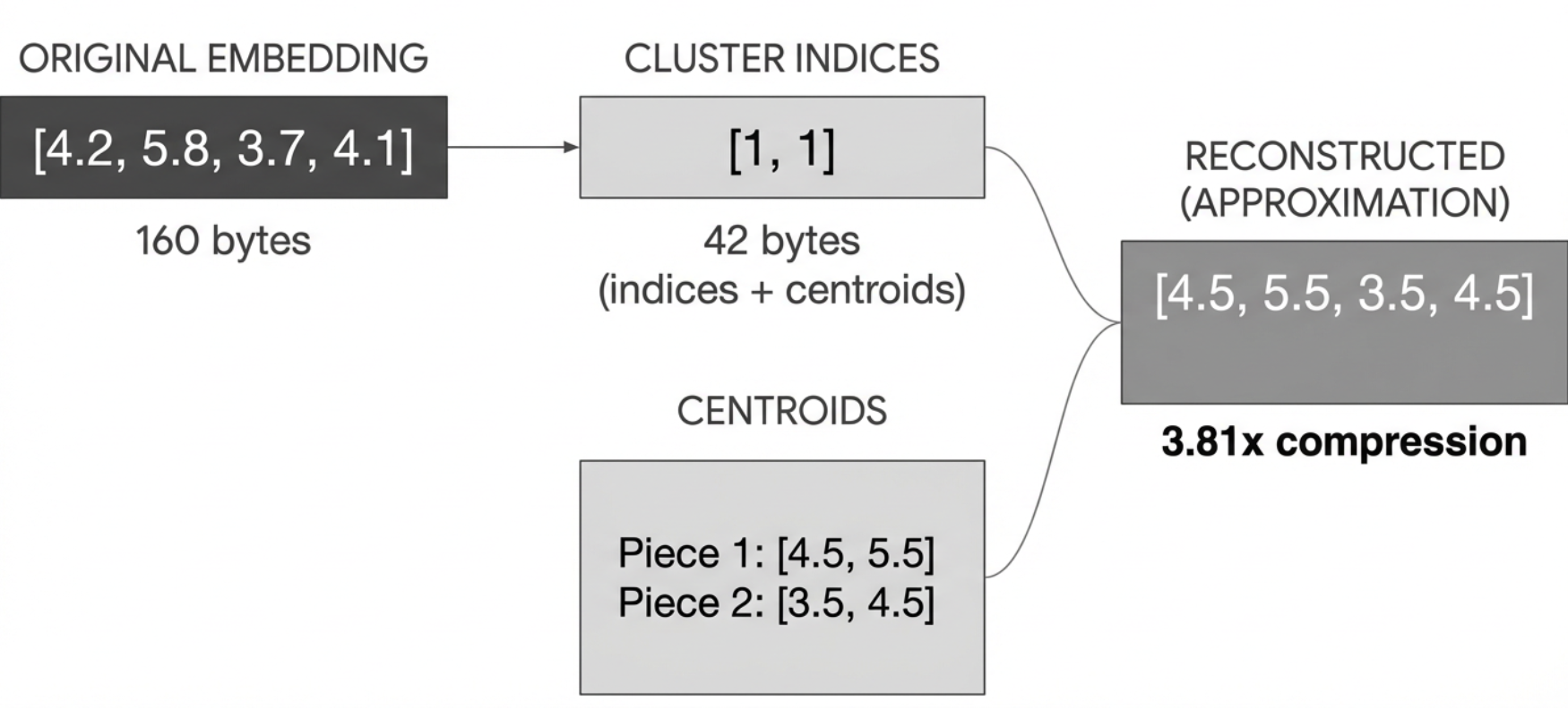
Step 4: Reconstruct by looking up centroids and combining.

To reconstruct an embedding, we look up the centroid for each piece and concatenate them. For example, embedding 1 has cluster index 1 for both pieces, so we look up centroids[0][1] = [4.5, 5.5] and centroids[1][1] = [3.5, 4.5], giving us [4.5, 5.5, 3.5, 4.5].

df = pd.DataFrame({
    'Embedding': [str(emb) for emb in embeddings],
    'Piece 1 Centroid': [centroids[0][idx] for idx in indices[0]],
    'Piece 2 Centroid': [centroids[1][idx] for idx in indices[1]]
})
concat_row = lambda row: np.concatenate([
    row['Piece 1 Centroid'], 
    row['Piece 2 Centroid']])
df['reconstructed'] = df.apply(concat_row, axis=1)
df

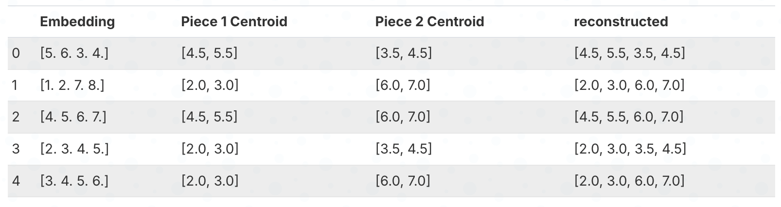
The reconstructed embeddings are not exactly the same as the originals. But we’ve compressed the data significantly by storing only cluster indices instead of the original numbers.

We can calculate the compression ratio to show that we are using less space even in this simple example.

# Calculate compression ratio
original_size = embeddings.nbytes
centroids_size = sum(c.nbytes for c in centroids)
indices_size = sum(i.nbytes for i in indices)
total_size = centroids_size + indices_size
compression_ratio = original_size / total_size

Compression Statistics:
Original size: 160 bytes
Total size after PQ: 42 bytes
Compression ratio: 3.81x

Overview

To summarize, the steps of product quantization are:

• Split each embedding into pieces
• Cluster each collection of pieces separately
• Store the centroid for each cluster
• Store which cluster each piece belongs to
• Reconstruct by looking up centroids and concatenating them

In the real implementation, we:

• Have many more embeddings (100,000+)
• Have many more dimensions (128)
• Use many more pieces (32)
• Have many more groups per piece (256)

But the basic idea is the same!

Real Implementation

Let’s start with creating a larger synthetic dataset to demonstrate the compression at a more realistic scale. Product quantization shines with lots of similar vectors, so we need a bigger dataset to see benefits to the compression ratio.

💡 While this quantization only working well with lots of similar may sound like it only works in specific cases, that specific case is always true in practice. Any dataset worth retrieving from is full of similar vectors based on topics within the dataset domain.

# Standard BERT embedding dimension
embedding_dim = 128  

# Create 10 topic clusters with varying sizes 
# to simulate a real dataset
n_topics = 10
topic_sizes = np.random.randint(5000, 15000, size=n_topics)
topic_centers = np.random.randn(n_topics, embedding_dim)

def embedding_func(i):
    return topic_centers[i] + np.random.randn(topic_sizes[i], embedding_dim) * 0.1

embeddings = np.vstack(parallel(embedding_func, list(range(n_topics)))).astype(np.float32)
norms = np.sqrt(np.sum(embeddings**2, axis=1, keepdims=True))
embeddings = embeddings / norms
embeddings_size_mb = embeddings.nbytes / (1024 * 1024)
n_vectors = embeddings.shape[0]
print(f"Size of embeddings: {embeddings_size_mb:.2f} MB")
print(f"{embeddings.shape=}")

Size of embeddings: 52.87 MB
embeddings.shape=(108275, 128)

We’ve created a dataset of embeddings of dimension 128, but instead of all random numbers, each embedding is a combination of a topic and a random noise vector. This is a much more realistic dataset and closer to what you would see in practice.

Example: If you are retrieving legal documents, you might have a topic like “Patent” and a random noise vector that represents the specific patent. The documents about Patents will typically have more similarity to each other than they do to documents about criminal law. However, each patent is different and so will have a different noise vector to represent that. This synthetic dataset loosely mimics 10 different topics with varying sizes like you would see in practice.

Let’s quantize these embeddings. All we need to do is refactor the code from the previous example to handle more data, more groups, and more dimensions!

Instead of splitting the embeddings in half, let’s make a flexible function that allows us to choose how many pieces we want to split the embeddings into.

def split_embeddings(embeddings, n_pieces):
    pieces_dim = embedding_dim // n_pieces
    pieces = []
    for i in range(n_pieces):
        piece_start = i * pieces_dim
        piece_end = (i + 1) * pieces_dim
        pieces.append(embeddings[:, piece_start:piece_end])
    return pieces, pieces_dim

pieces, pieces_dim = split_embeddings(embeddings, 16)

Here we split the embeddings into 32 pieces. Each piece has the first 8 dimensions of the embeddings.

pieces[0].shape=(108275, 8) pieces_dim=8

Next we need to find the groups for each piece. We’ll do this the same way we did in the previous example, but make a more flexible function so we’ll have some parameters to play with and we can put it on a GPU if we want.

Because we’re using the fastkmeans library we can easily put it on a GPU to make it run faster so lets allow these parameters to be set. fastkmeans is a very fast implementation of kmeans by Ben Clavié and Benjamin Warner that is done properly and does not have painful dependencies. This is a big deal.

def train_kmeans(piece, k, n_iter=20, nredo=1, gpu=False, use_triton=False):
    kmeans = FastKMeans(d=piece.shape[1], k=k, nredo=nredo, niter=n_iter, gpu=gpu, use_triton=use_triton)
    kmeans.train(piece)
    return kmeans

centroids, indices = [], []
for piece in pieces:
    kmeans = train_kmeans(piece, k=256) # 256 groups per piece
    centroids.append(kmeans.centroids)
    indices.append(kmeans.predict(piece).astype(np.uint8))

Let’s calculate the compression ratio to see how much space we’ve saved for this dataset.

original_size = embeddings.nbytes
centroids_size = sum(c.nbytes for c in centroids)
indices_size = sum(i.nbytes for i in indices)
total_size = centroids_size + indices_size
compression_ratio = original_size / total_size

Compression Statistics:
Original size: 55436800 bytes
Total size after PQ: 1863472 bytes
Compression ratio: 29.75x

Quite a lot better than the 8x we got with the scalar quantization!

Now that we have our compressed embeddings, we can reconstruct them. Let’s do that so we can measure the error.

def reconstruct_embeddings(centroids, indices):
    reconstructed = np.zeros_like(embeddings)
    for i, piece in enumerate(pieces):
        reconstructed[:, i*pieces_dim:(i+1)*pieces_dim] = centroids[i][indices[i]]
    return reconstructed

We can calculate the compression ratio to show that we are using less space, even in this simple example.

Let’s calculate the error on a sample of the data.

sample_size = 1000
error_sum = 0

for i in range(sample_size):
    idx = np.random.randint(0, n_vectors)
    sample_reconstructed = reconstruct_embeddings(centroids, [indices[i][idx:idx+1] for i in range(len(indices))])
    error_sum += np.mean(np.abs(embeddings[idx] - sample_reconstructed[0]))

print(f"Mean absolute error: {error_sum / sample_size:.6f}")

Mean absolute error: 0.005148

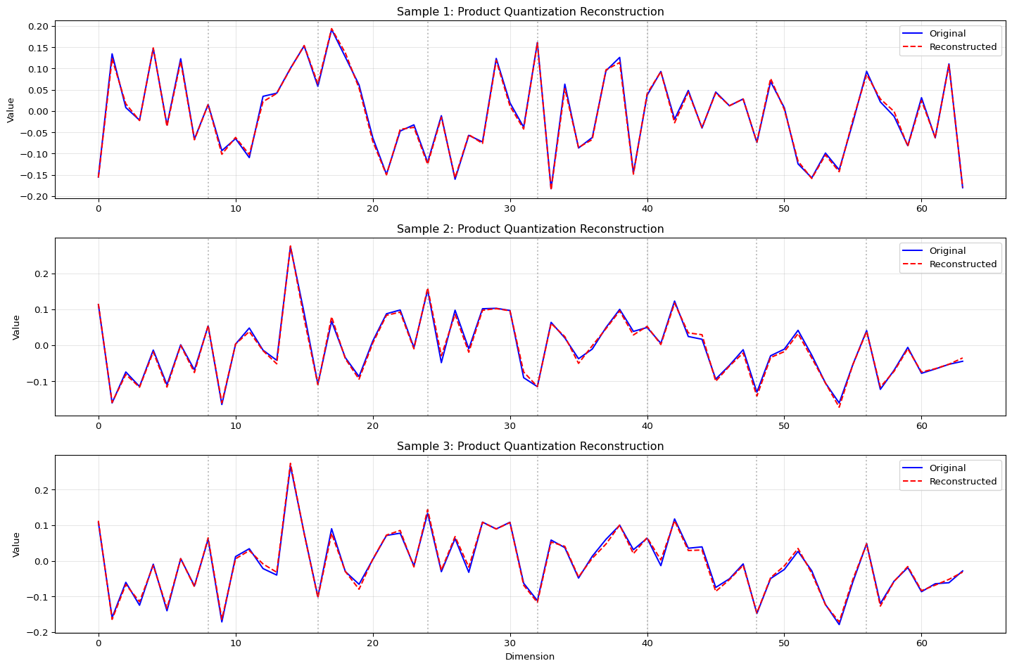
Let’s visualize multiple samples to get a better understanding of the reconstruction quality:

# Visualize multiple samples
plt.figure(figsize=(15, 10))

# Number of samples to show
n_viz_samples = 3
dims_to_show = 64  # Show more dimensions

for plot_idx in range(n_viz_samples):
    # Get a random sample
    sample_idx = np.random.randint(0, n_vectors)
    original = embeddings[sample_idx]
    reconstructed = reconstruct_embeddings(centroids, [indices[i][sample_idx:sample_idx+1] for i in range(len(indices))])[0]
    
    # Create subplot
    plt.subplot(n_viz_samples, 1, plot_idx+1)
    x = np.arange(dims_to_show)
    plt.plot(x, original[:dims_to_show], 'b-', label='Original')
    plt.plot(x, reconstructed[:dims_to_show], 'r--', label='Reconstructed')
    
    # Add vertical lines at subvector boundaries
    for i in range(1, len(pieces)):
        boundary = i * pieces_dim
        if boundary < dims_to_show:
            plt.axvline(x=boundary, color='grey', linestyle=':', alpha=0.5)
    
    plt.title(f'Sample {plot_idx+1}: Product Quantization Reconstruction')
    plt.ylabel('Value')
    if plot_idx == n_viz_samples-1:
        plt.xlabel('Dimension')
    plt.legend()
    plt.grid(True, alpha=0.3)

plt.tight_layout()
plt.show()

Extreme Quantization

We’ve seen how product quantization can give us great compression ratios while maintaining good quality. But what if we want to go even further? That’s where extreme quantization comes in.

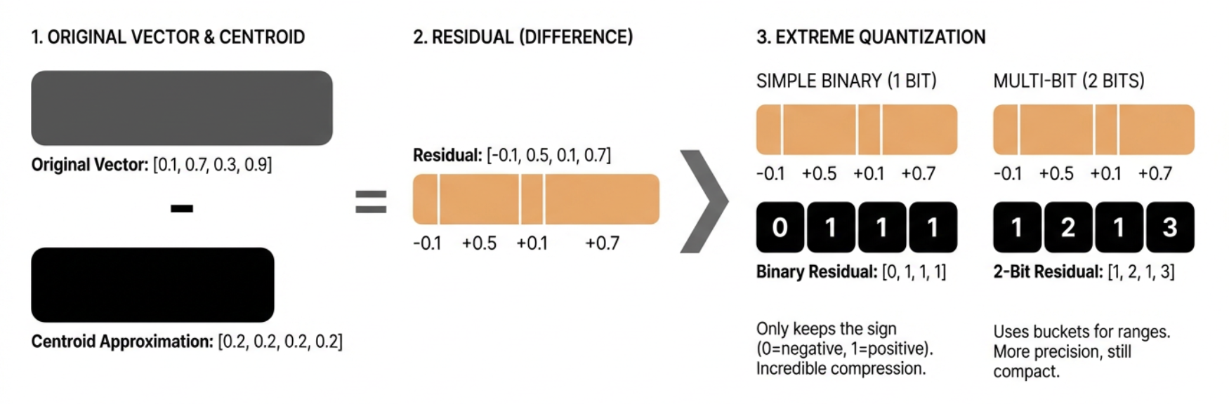
The key insight is that after product quantization, we still have some information left in the original vectors that we haven’t captured. We can capture this “residual” information using an even more aggressive form of quantization.

Let’s start with a simple example to understand the concept:

# Create a small example to demonstrate extreme quantization
original = np.array([0.1, 0.7, 0.3, 0.9])
centroid = np.array([0.2, 0.2, 0.2, 0.2])
residual = original - centroid
print(f"Original: {original}")
print(f"Centroid: {centroid}")
print(f"Residual: {residual}")

Original: [0.1 0.7 0.3 0.9]
Centroid: [0.2 0.2 0.2 0.2]
Residual: [-0.1  0.5  0.1  0.7]

The residual is what’s left after we subtract the centroid from the original vector. In our case, it’s the difference between our product quantized approximation and the true vector.

Now, instead of storing these residuals as full floating-point numbers, we can quantize them extremely aggressively. One way to do this is to use binary quantization (represent each value with a single bit).

Here’s how we can do binary quantization:

def simple_binary_quantize(residual):
    # Convert to binary: 1 if positive, 0 if negative
    return (residual > 0).astype(np.uint8)

binary_residual = simple_binary_quantize(residual)
print(f"Binary residual: {binary_residual}")

Binary residual: [0 1 1 1]

This is extremely aggressive - we’re only keeping the sign (positive or negative) of each number! But when combined with product quantization, it can still be useful because:

• The product quantization already captures most of the important information
• The residual is usually small, so just knowing its sign can be helpful
• We get incredible compression - just 1 bit per dimension!

In practice, we can be a bit more sophisticated. Instead of just using 1 bit, we can use multiple bits to represent different ranges of values. This gives us more precision while still maintaining good compression.

Here’s a more advanced version that uses multiple bits:

def multi_bit_quantize(residual, n_bits=2):
    # Create buckets for different ranges
    max_val = np.max(np.abs(residual))
    buckets = np.linspace(-max_val, max_val, 2**n_bits)
    
    # Assign each value to a bucket
    quantized = np.digitize(residual, buckets) - 1
    return quantized.astype(np.uint8)

# Try with 2 bits (4 buckets)
two_bit_residual = multi_bit_quantize(residual, n_bits=2)
print(f"2-bit residual: {two_bit_residual}")

2-bit residual: [1 2 1 3]

This approach gives us more precision while still maintaining good compression. We can choose how many bits to use based on our needs:

• More bits = better precision but more storage
• Fewer bits = worse precision but less storage

The actual implementation in ColBERT uses a similar approach but with some optimizations:

• It uses bit packing to store the quantized values efficiently
• It handles the quantization in chunks to work with GPU memory efficiently
• It includes special handling for edge cases and different data types

The key insight is that by combining product quantization with extreme quantization of the residuals, we can get even better compression ratios while maintaining good quality. The product quantization captures the main structure of the vectors, while the extreme quantization of residuals captures the fine details.

This is particularly useful in ColBERT because:

1. It allows storing more token embeddings in memory
2. It enables faster similarity calculations
3. It maintains good retrieval quality despite the aggressive compression

The tradeoff is that we need to do more computation to reconstruct the vectors, but this is usually worth it for the space savings we get.

The Real ColBERT Approach

Now that we understand the basic concept, let’s look at how ColBERT actually implements extreme quantization. The real implementation is more sophisticated and efficient than our simple examples.

Here’s the actual code used in ColBERT:

def binarize(self, residuals):
    # Convert residuals to buckets based on their values
    residuals = torch.bucketize(residuals.float(), self.bucket_cutoffs).to(dtype=torch.uint8)
    
    # Expand to add a new dimension for each bit we'll use
    residuals = residuals.unsqueeze(-1).expand(*residuals.size(), self.nbits)
    
    # Right shift to get each bit in position
    residuals = residuals >> self.arange_bits
    
    # Keep only the least significant bit
    residuals = residuals & 1

    # Ensure dimensions are compatible with bit packing
    assert self.dim % 8 == 0
    assert self.dim % (self.nbits * 8) == 0, (self.dim, self.nbits)

    # Pack bits into bytes for efficient storage
    if self.use_gpu:
        residuals_packed = ResidualCodec.packbits(residuals.contiguous().flatten())
    else:
        residuals_packed = np.packbits(np.asarray(residuals.contiguous().flatten()))
    
    # Convert back to tensor and reshape to final form
    residuals_packed = torch.as_tensor(residuals_packed, dtype=torch.uint8)
    residuals_packed = residuals_packed.reshape(residuals.size(0), self.dim // 8 * self.nbits)

    return residuals_packed

Let’s break down how this works:

• Bucketization: First, we convert the residual values into buckets using torch.bucketize. This is similar to our multi_bit_quantize function but more efficient. The bucket_cutoffs define the boundaries between different values.
• Bit Expansion: We expand the bucketed values to add a new dimension for each bit we’ll use. This is where we prepare to extract individual bits from each value.
• Bit Extraction: The >> (right shift) operation moves each bit into position, and the & 1 operation keeps only the least significant bit. This effectively converts each value into its binary representation.
• Bit Packing: Finally, we pack these bits into bytes for efficient storage. This is where we get our extreme compression - we’re storing multiple values in a single byte!

Let’s see this in action with a small example:

# Create a small example to demonstrate the real approach
import torch
import numpy as np

# Create some example residuals
residuals = torch.tensor([[0.1, 0.7, 0.3, 0.9],
                         [0.2, 0.5, 0.8, 0.4]])

# Define bucket cutoffs (simplified for example)
bucket_cutoffs = torch.tensor([0.0, 0.3, 0.6, 0.9])

# Step 1: Bucketize
buckets = torch.bucketize(residuals, bucket_cutoffs).to(dtype=torch.uint8)
print(f"After bucketization:\n{buckets}")

# Step 2: Expand for bits
nbits = 2  # Using 2 bits per value
expanded = buckets.unsqueeze(-1).expand(*buckets.size(), nbits)
print(f"\nAfter expansion:\n{expanded}")

# Step 3: Extract bits
arange_bits = torch.arange(nbits, device=expanded.device)
bits = (expanded >> arange_bits) & 1
print(f"\nAfter bit extraction:\n{bits}")

# Step 4: Pack bits
packed = np.packbits(bits.numpy().flatten())
packed = torch.from_numpy(packed).reshape(bits.size(0), -1)
print(f"\nFinal packed form:\n{packed}")

# After bucketization:
tensor([[1, 3, 1, 3],
        [1, 2, 3, 2]], dtype=torch.uint8)

# After expansion:
tensor([[[1, 1],
         [3, 3],
         [1, 1],
         [3, 3]],

        [[1, 1],
         [2, 2],
         [3, 3],
         [2, 2]]], dtype=torch.uint8)

# After bit extraction:
tensor([[[1, 0],
         [1, 1],
         [1, 0],
         [1, 1]],

        [[1, 0],
         [0, 1],
         [1, 1],
         [0, 1]]])

# Final packed form:
tensor([[187],
        [157]], dtype=torch.uint8)

The key differences from our simplified version are:

• Bucketization: We use torch.bucketize instead of multi_bit_quantize
• Bit Expansion: We expand the bucketed values to add a new dimension for each bit we’ll use
• Bit Extraction: We extract individual bits from each value
• Bit Packing: We pack these bits into bytes for efficient storage

This is the actual implementation used in ColBERT. It’s more sophisticated and efficient than our simple examples.